Background Info

Exercise – Vibrational Spectroscopy using Nuclear Wave Functions

The simplest way to generate vibrational spectra is the harmonic approximation: all second derivatives of the energy with respect to the nuclear degrees of freedom are computed at a pre-optimized minimum structure, yielding the Hessian: \[ H_{ij} = \frac{\partial^2 \left < E \right > }{\partial q_i \partial q_j} \] After extraction of the force constants \(k\) of each vibrational mode from the Hess-matrix (via diagonalisation), the harmonic frequencies \(\nu\) can be obtained via

\[ \nu = \frac{1}{2\pi} \sqrt{\frac{k}{\mu}} \]

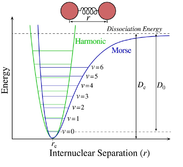
with \(\mu\) being the associated reduced mass. However, a short-coming of this approach is the neglect of anharmonicity, mode coupling and nuclear quantum effects. In some cases these contributions cancel, while for other systems the error in the harmonic frequencies can be up to \(300\,\mathrm{cm^{-1}}\).

An elegant alternative is the calculation of vibrational wave functions by numerically solving the nuclear Schrödinger equation. One method to achieve this is a method according to Boris V. Numerov requiring the potential curve as input in form of a discretised grid. The latter can be obtained from a potential energy scan executed for instance using the QM program gaussian. The difference between the eigenvalue of the ground state (\(n=0\)) and the first (\(n=1\)) and second (\(n=2\)) excited states correspond to the expected vibrational frequency of the fundamental and first overtone, when divided by Planck’s constant:

\[ \nu_{n0} = \frac{E_n - E_0}{h} \]

From the frequencies \(\nu_{n0}\) (in \(\mathrm{s}^{-1}\)) the respective wave numbers \(\bar{\nu}_{n0}\) (in \(\mathrm{cm}^{-1}\)) have to be calculated and reported. Knowledge of the wave function also enables the calculation of the oscillator strengths \(f_{n0}\), providing an accurate estimate of the expected IR absorption intensities.

\[ f_{n0} = \frac{4\pi m_{\mathrm{e}}}{3\mathrm{e}^2\hbar c}|\mu_{n0}|^2 \bar{\nu}_{n0}= 4.702 \cdot 10^{-7}\,\mathrm{\frac{cm}{D^2}}|\mu_{n0}|^2 \bar{\nu}_{n0} \]

To calculate the oscillator strength, the wave numbers \(\bar{\nu}_{n0}\) and the respective transition dipole moment \(\mu_{n0}\) is required. The latter is given as:

\[ |\mu_{n0}|^2 = |\mu_{n0}^x|^2 + |\mu_{n0}^y|^2 + |\mu_{n0}^z|^2 \]

with

\[ |\mu_{n0}^x| = \left < \psi_0 | \mu^x | \psi_n \right > = \int_{-\infty}^{\infty} \psi_0 \mu^x \psi_n dx \]

While this integral appears intimidating, it can be easily evaluated in an approximate way using the trapezoidal rule:

\[ \int_a^b f(x) dx \approx \frac{\Delta x}{2} (y_1 + 2y_2 +2 y_3+ ... + 2y_{n-1}+y_n) \] \[ \approx \frac{\Delta x}{2} \sum_{i=1}^{n-1} (y_i + y_{i+1}) \]

The calculation of the trapezoidal integration is actually very simple and can be easily implemented in a spreadsheet editor such as libreoffice or excel (or computed using data science software such as matlab, octave,python, R, etc.)

Diatomic molecule

In this part the vibration of a diatomic molecule is investigated. After drawing the molecule using gaussview, an energy minimisation (= geometry optimisation) and a harmonic frequency calculation has to be carried out. In the next step a potential energy scan has to be performed in the range of approx. -0.5\(\,\)Å to +1.5\(\,\)Å using a step length \(\Delta r = 0.01\,\)Å. This yields about \(150\) individual potential points.

The energy and dipole moment information can be extracted in the terminal using the provided tool:

./extract_data.sh  scan-logfile   >  data-file

The data file contains the distance information in Å, the QM energy in Hartree, and the components of the dipole moment in \(x\), \(y\) and \(z\) direction in Debye. Next, the force constant \(k\) according to the harmonic approximation has to be determined via finite differences from the energy column of the data-file (second column).

\[ k \approx \frac{E_1 -2 E_{\mathrm{min}} + E_{+1}}{\Delta r^2} \]

with \(E_{\mathrm{min}}\) being the minum energy and \(E_{\pm 1}\) corresponding to the energy values of the two neighbouring points. Please report the force constant in \(\mathrm{kcal\cdot mol^{-1}Å^{-2}}\):

Because the program gaussian provides a wrong reduced mass \(\mu\) in case of diatomic systems, this property has to be calculated manually in this part of the exercise.

\[ \mu = \frac{m_1 m_2}{m_1+m_2} \]

Using the reduced mass \(μ\) and the force constant \(k\) the frequency (in \(\mathrm{s^{-1}}\)) and corresponding wave number (in \(\mathrm{cm^{-1}}\)) should be calculated and compared to the result obtained from gaussian.

Note

Extra care is required to apply all factors to obtain the correct unit of the frequency and wavenumber (i.e. just dividing the force constant \(k\) in \(\mathrm{kcal\cdot mol^{-1}Å^{-2}}\) by the reduced mass \(\mu\) given in \(\mathrm{g \cdot mol^{-1}}\) will obviously yield a wrong result …)

In the final step the Numerov calculation is carried out, requiring the data file and the reduced mass as input:

./numerov    data-file   mass   >  numerov-outfile

The output of the Numerov procedure contains the coordinate and potential information (in units Å and \(\mathrm{kcal\cdot mol^{-1}}\)) as well as the wave-functions for the five lowest states. The energy eigenvalues are given as comment line (also in \(\mathrm{kcal\cdot mol^{-1}}\)) on top of the Nuermov output file. The respective energy differences have to be transformed into \(\mathrm{cm^{-1}}\).

The report for this part should include:

A screenshot of the equilibrium geometry (white background!).
The calculation of the force constant \(k\) and the reduced mass \(\mu\).
Calculation of the frequency and wave number showing ALL(!) required conversion factors.
A figure showing the QM energy as a function of distance and the Numerov wave functions plus the energy graph showing the harmonic approximation (all in the same figure).
A table comparing the wavenumbers obtained via the Numerov procedure with the results obtained from the harmonic approximation for \(n\) = 1 - 4.
For all points a short description/interpretation should be included as text.

Note

In this part, the transition dipole moments and oscillator strengths are NOT(!) required.

Stretch Vibration in a Polyatomic Molecule

In this example, the X-H stretch motion of a polyatomic molecule (X=O,N) provides a suitable approximation to the actual normal mode. In order to assess the influence of quantum effects, both hydrated and deuterated species (i.e. X-H and X-D) have to be investigated. After the geometry optimisation and frequency computation, the potential energy scan of the X-H distance in the range of approx. \(0.5\,\mathrm{Å}\) to \(2.0\,\mathrm{Å}\) has to be carried out, using again a step length of \(0.01\,\mathrm{Å}\).

Careful:

Be sure to select the correct bond for the potential energy scan! (This is a very frequent error in this excercise.)

As before the energy and dipole moment information can be extracted in the terminal using the provided tool:

./extract_data.sh    scan-logfile     >    data-file

The resulting data file contains the coordinate, energy and dipole moment information (in units of Å, Hartree and Debye) and can be directly used as input for the Numerov programm:

./numerov    data-file   mass   > numerov-outfile

In addition to the data file, the reduced mass of the vibrational mode has to be provided as a second input. For polyatomic molecules the reduced mass provided in the gaussian output file is correct! To identify the correct mode, a visual inspection in gaussview is required.

Careful:

Be sure to make a separate check in the deuterated case – the order of vibrations is sometimes different (again a very common error in this excercise).

As before the output of the Numerov procedure contains the coordinate and potential information (in units Å and \(\mathrm{kcal\cdot mol^{-1}}\)) as well as the wave-functions for the five lowest states. The energy eigenvalues are given as comment line (also in \(\mathrm{kcal\cdot mol^{-1}}\)) on top of the file. The respective energy differences have to be transformed into \(\mathrm{cm^{-1}}\). Prior to computing the transition dipole moments it should be verified that the wave functions are orthonormal for the states \(i, j\) = 0 – 2.

\[ \left < \psi_i | \psi_j \right > - \delta_{ij} = 0 \]

Next, the oscillator strength \(f_{n0}\) (for \(n=1,2\)) should be computed from the transition dipole moments and reported relative to \(f_{10}\). (i.e. the oscillator strengths are divided by \(f_{10}\), thus always giving a number of \(1.0\) for the ground state transition).

The report for this part should include:

A screenshot of the equilibrium geometries (white background!).
Two figures comparing the potential energy and the first five wave functions including also the potential energy of the harmonic approximation for both the hydrated and deuterated species.
A graph showing the components of the dipole moment as a function of the distance.
Results of the orthonormality check between the states \(i\), \(j = {0,1,2}\) in form of a table.
A table comparing the frequencies and oscillator strengths of the fundamental and first overtone modes obtained via the Numerov procedure and the harmonic approximation.
For all points a short description/interpretation should be included as text.

Protocol:

The protocol in this section should be designed as an A0-Poster (similar to those Ph.D. students typically prepare for their presentations in the Atrium of the CCB building), see poster templeates. All data generated along with a discussion of results fit easily on a single page. Please include your name and matriculation number, and provide the protocol as pdf-file including your surname in the name of the file.