You can also grep for this statement to verify the normal termination of the simulation for all files:
grep "PQ ended" *.log
Visual inspection
Check if the system is behaving as expected.
Open the *.xyz file with VMD.
It is a good sign if
Troubleshooting
In the event that the simulation does not produce the anticipated results:
etc.
Equilibrium state of simulation
Firstly, in order to obtain meaningful physical properties from a simulation, it is essential to ensure that the system is in an equilibrium state. However, what constitutes an equilibrium state?
ImportantAn equilibrium state:
can be defined as a state in which macroscopic properties \(A\) (e.g temperature \(T\), pressure \(P\), energies \(E\), volume \(V\), …) do NOT undergo major changes over time.
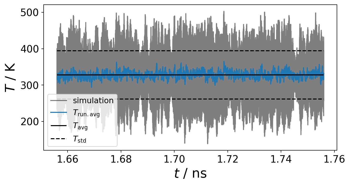
Once these properties fluctuate around a constant pattern without any long-term trends, it can be assumed that the system reached an equilibrium state.
Arithmetic Average, Standard Deviation and Standard Error
The aforementioned constant relaxation of the properties can be verified by calculating the arithmetic mean of the properties \(\left < A \right >\)
\[
\left < A \right > = \frac{1}{n}\sum_{i=0}^{n} a(t_{i})
\] where \(a(t_{i})\) is the property \(a\) at time step \(t_i\) and \(n\) the total sampling time
as well as the standard deviation \(A_{\sigma }\)
\[
A_{\sigma }= \sqrt{ \frac{1}{n}\sum_{i=0}^{n} (a(t_{i}) - \left < A \right > )^2}.
\] and standard error \(A_{\nu}\) of the arithmetic average \[
A_{\nu} = \frac{A_{\sigma }}{\sqrt{n}}
\]
Running Average
Further, the running average \(\left < A \right >_{\tau}\) at time \(\tau\) with a window size of \(\omega\) and a gap size \(g\)
can help to estimate the fluctuation of the properties over time.
Cumulative Average
And the cumulative average is a running average that is added at each step. \[
\left < A \right >_n = \frac{(n-1)\left < A \right >_{n-1} + \left < A \right >_n}{n}
\]
Linear Regression Fit
A linear regression fit can help to estimate the trend of your simulation.
The temperature during the simulation can be found in the associated energy file *.en, which can be readily used for plotting. The *.info file contains information about the individual columns in the *.en file. An example code to plot the temperature vs simulation time is shown below.
The thermal expansion coefficient is a quantity that describes the extent to which a solid substance undergoes a change in size in response to variations in temperature.
Therefore the system is computed in the \(NPT\) ensemble at different temperatures \(T_i\) at \(1\,\mathrm{bar}\).
In our case we consider a temperature range from \(248\,\text{to}\,348\,\mathrm{K}\) in \(25\,\mathrm{K}\) steps.
Linear thermal expansion coefficient
The linear thermal expansion coefficient at \(\mathrm{298}\,\mathrm{K}\) is calculated from the temperature gradient of the respective average lattice parameter \(\left < a \right >\), \(\left < b \right >\) or \(\left < c\right >\) at constant pressure \(P\) (\(NPT\) ensemble). \[
\alpha _{x}^{T_{\mathrm{298\,K}}} = \frac{1}{x} \left ( \frac{\partial x}{\partial T} \right ) _{P}, x={a,b,c}
\] The slope can be estimated numerically in different ways. A simple way is to employ a finite difference method. There are three fundamental types of finite differentiation: forward, backward and central finite differentiation.
We will use the central finite difference method with a five-point stencil. In general it is formulated in 1D as: \[
f'(x) = \frac{-f(x+2h)+8f(x+h)-8f(x-h)+f(x-2h)}{12 h} + \frac{h^4}{30}f^{(5)(c)}, c \in [x-2h,x+2h]
\] where \(h\) is the change of \(x\).
If you use more than five points, a higher order stencil can be used.
In our case the differentiation can be written as: \[
\frac{\partial x}{\partial T} \approx \frac{ \left < x^{T_{\mathrm{248\,K}}}\right >-8 \left < x^{T_{\mathrm{273\,K}}}\right > + 8 \left < x^{T_{\mathrm{323\,K}}}\right > - \left < x^{T_{\mathrm{348\,K}}} \right > }{12\Delta T}
\]
Volumetric thermal expansion coefficient It is the same formulation as for the linear thermal expansion coefficient, except that the volume \(V\) is used instead of the individual lattice parameters:
The volume of a orthorhombic system can be calculated as: \[
V = a\cdot b \cdot c
\] In general, the volume of a non-orthorhombic crystal systems is calculated as: \[
V = a b c \sqrt{1-\mathrm{cos}^2(\alpha) -\mathrm{cos}^2(\beta) - \mathrm{cos}^2(\gamma)+ 2(\mathrm{cos}(\alpha) \mathrm{cos}(\beta) \mathrm{cos}(\gamma))}
\]
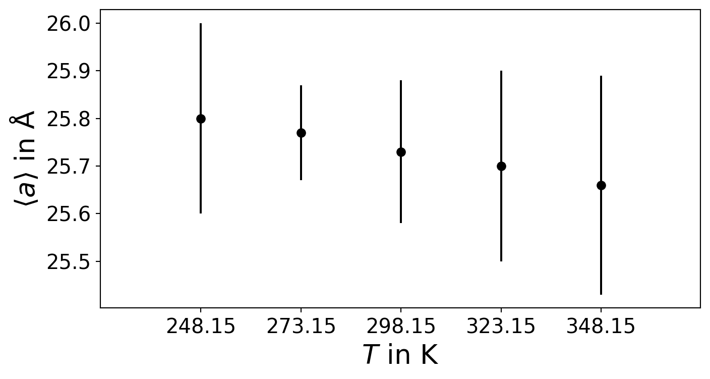
Plot Lattice Parameter vs. Temperature
Code
import numpy as npimport matplotlib.pyplot as pltimport matplotlib as mplmpl.rcParams["font.size"] =15mpl.rcParams["axes.labelsize"] =20temperature = np.array([248.15,273.15,298.15,323.15,348.15])a = np.array([25.8, 25.77, 25.73, 25.70, 25.66])a_err = np.array([0.2,0.1,0.15,0.2,0.23])plt.figure(figsize=(8,4))plt.errorbar(temperature,a,a_err,fmt='ok',label=r"$\left < a \right >$")plt.xlabel(r"$T$ in K")plt.ylabel(r"$\left < a \right > $ in $\mathrm{\AA}$")plt.xlim(223,373)plt.xticks(temperature)# plt.legend(fontsize=12)plt.show()
Figure 7.2: T vs a plot
NoteExperimental Measurement Data is available from:
X-ray Diffraction (XRD)
Powder X-ray Diffraction (PXRD)
Neutron Powder Diffraction (NPD)
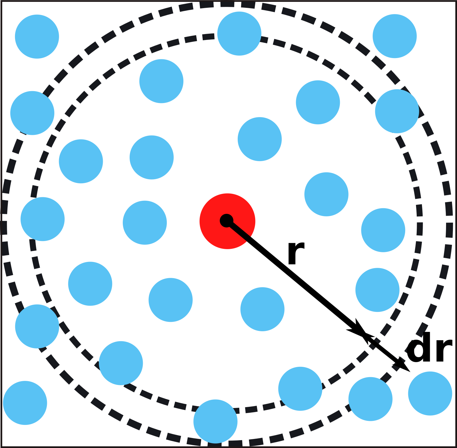
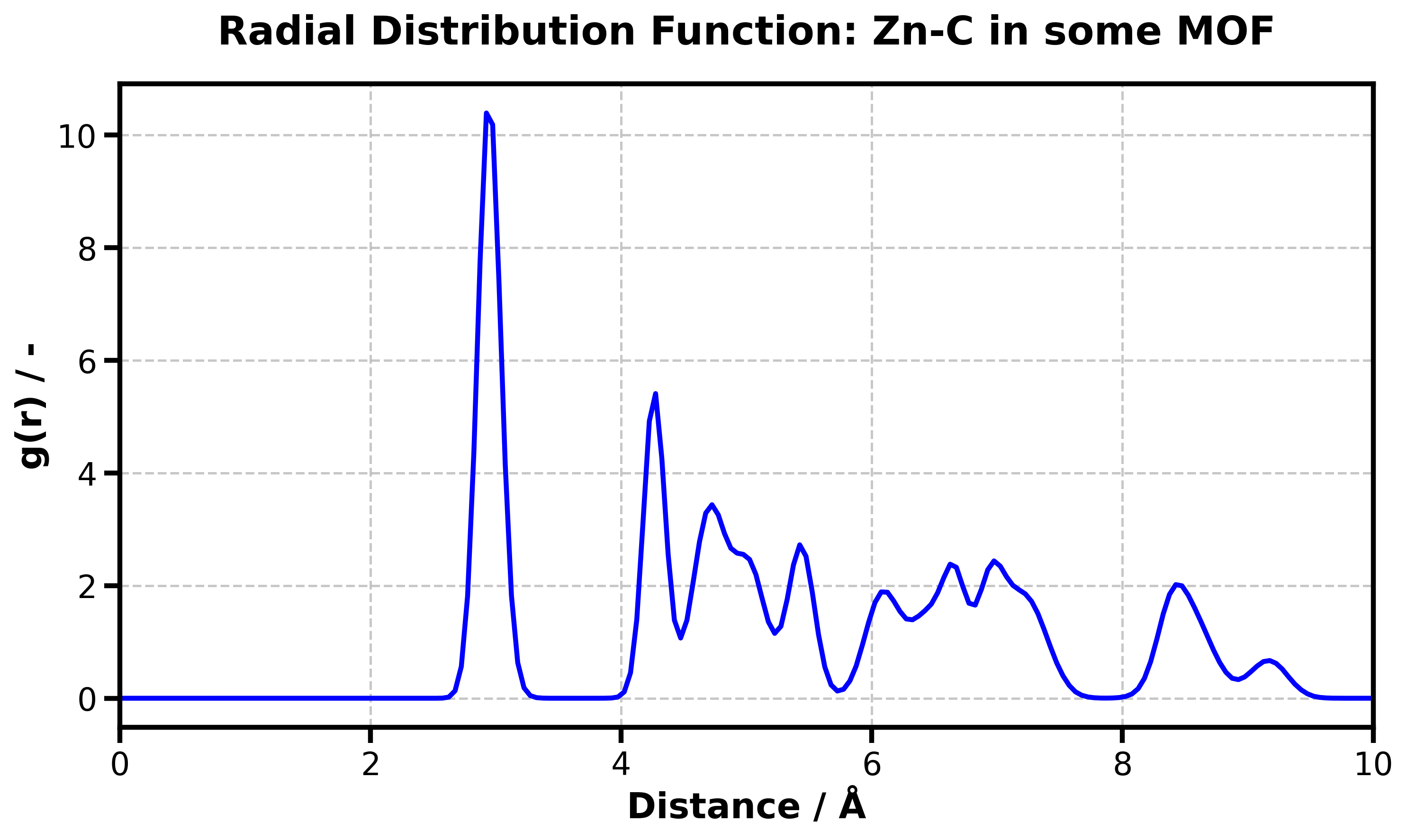
Radial Distribution Functions (RDFs)
The radial distribution function (RDF) is a simple measurement to get structural information of the system.
It describes the probability \(P_{ab}(r)\) to find a target particle type \(b\) at distance \(r\) away from a reference particle type \(a\); e.g. the probability to find \(\mathrm{C}\mathrm{O}_2\) from \(\mathrm{Zn}^{2+}\) clusters at distance \(r\): \[
P_{ab}(r) = \int_{0}^{r'} 4\pi r'^2 g_{ab}(r') dr'
\] where \(g_{ab}(r)\) is the RDF. The RDF formulates the average local density \(\left <\rho_{ab}(r)\right >\) normalized by \(\rho=(N_a N_b)\)\[
g(r) = \frac{\left <\rho_{ab}(r)\right >}{\rho}.
\]
The two-particle density correlation function is defined as:
The average number of particles \(b\) that can be found in the shell of distance \(r\) can be determined by multiplying the density \(\rho\) with the probability \(G(r)\)\[
N_{ab}(r) = \rho G_{ab}(r)
\]
TipDirac-Delta Function
\[
\delta(x-x_0) = \begin{cases}
0 & x \neq x_0\\
\infty & x = x_0\\
\end{cases}
\]\[
\int_L \delta(x-x_0) dx = 1, x_0 \in L
\]
Self-Diffusion Coefficient
In order to describe the dynamic of guests in host systems, it is necessary to calculate transport properties. A transport property would be for example the diffusion, viscosity, electrical or thermal conductivity.
In general, transport properties can be described as a property coefficient \(\gamma\) which depends on microscopic variable \(A\) (e.g. positions \(\Delta \vec{r}\) or the velocities \(\vec{v}\)) that is written as an infinite time integration of a non-normalized time correlation function \(\left < \dot{A}(t)\dot{A}(t_0) \right >\) : \[
\gamma = \int_{0}^{\infty} dt \left < \dot{A}(t)\dot{A}(t_0) \right >.
\] This is also known as Green-Kubo relation1 which can also written as the equivalent Einstein expression
In case of self-diffusion coefficient \(D_{\mathrm{s}}\) the variable \(A\) is the molecular position \(\vec{r}_{\mathrm{cm}}\) which in general is the center of mass position of the particles: \[
\vec{r}_{\mathrm{cm}} = \frac{\sum_{i=1}^{N} m_i \vec{r}_i}{\sum_{i=1}^{N} m_i}
\] where \(m_i\) is the atomic mass, \(\vec{r}_i\) is the atomic positions and \(N\) the number of atoms in the particle.
As well as \(\dot{A}\) is the molecular velocity which should be also considered as center of mass.
Einstein-Relation
The Einstein Relation can be therefore written as slope of the mean-squared-displacement (\(MSD(\tau)\)) over time origins \(\tau\)
\[
D_{\mathrm{s}} = \frac{1}{2 \cdot d} \lim _{t\to \infty} \frac{d}{dt} MSD(\tau)
\] where \(d=1,2,3\) is the dimensionality.
Mean-Squared Displacement
The mean-squared displacement describes the temporal displacement of the particle from a time origin \(t_0\) averaged over the time interval \(\tau\)\[
MSD(\tau) = \left < \frac{1}{N} \sum_{i=1}^{N} |\vec{r} _{i}(t) - \vec{r} _{i}(t_0)|^2 \right >_{\tau}
\] where \(N\) is the number of the particle, \(\vec{r}_{i}\) is the center-of-mass position vector of the particle \(i\).
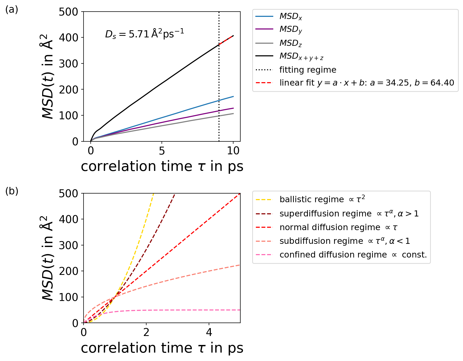
Looking at Figure Figure 7.3 (a), we see that the beginning of the MSD is not linear. Only at higher correlation times the expected diffusion (see Figure Figure 7.3 (b)) behaviour can be observed.
TipQuestion:
How do you get the self-diffusion coefficient out of the MSD regarding the Einstein-relation?
How do you get the gradient/slope of the MSD?
What does the limes in that formula mean?
CautionAnswer:
The self-diffusion coefficient is the slope of the MSD divided by 2 \(\cdot\;d\).
But this is only true if the correlation time is long enough. We can say that in the linear regime we fulfill this limes due to the constant slope, which represents the diffusion coefficient.
Therefore, in order to apply the Einstein relation, it is important to be in the linear regime of the MSD plot.
You get the slope by fitting a linear regression to the linear part of the dataset.
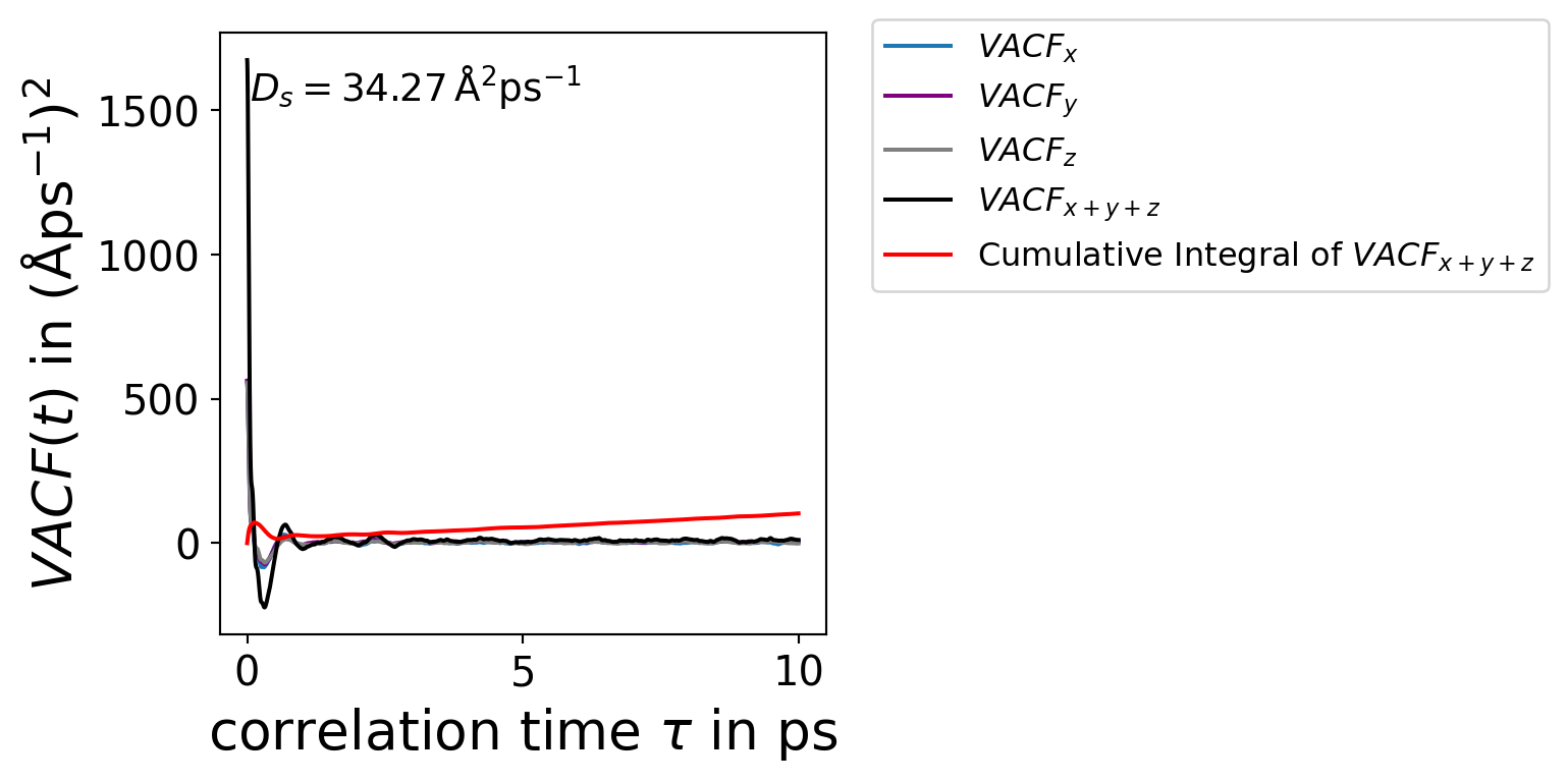
The Green-Kubo formalism needs a numerical integration of the velocity-autocorrelation function \(VACF(t)\) to get the self-diffusion coefficent \(D_{\mathrm{s}}\)\[
D_{\mathrm{s}} = \frac{1}{d} \int _{0}^{\infty} VACF(t) dt
\] where \(d=1,2,3\) is the dimension.
Veloctiy-Autocorrelation Function
The velocity-autocorrelation function\(VACF(\tau)\) is averaged over a time interval \(\tau\)\[
VACF(\tau) = \left < \frac{1}{N} \sum_{i=1}^{N} |\vec{v} _{i}(t) \vec{v} _{i}(t_0)|^2 \right >_{\tau}
\] where \(\vec{v}_{i}\) is the velocity of the particle \(i\) and \(t_0\) labels the time origin.
Code
import numpy as npimport matplotlib.pyplot as pltfrom scipy.integrate import simpsonfrom scipy.integrate import cumulative_trapezoidimport matplotlib as mplmpl.rcParams["font.size"] =15mpl.rcParams["axes.labelsize"] =20data = np.genfromtxt("../data/green_kubo.out")time = data[:,0]VACF_x = data[:,1]VACF_y = data[:,2]VACF_z = data[:,3]VACF_xyz = data[:,4]integral_VACF_xyz = simpson(VACF_xyz, x=time)cumulative_integral = cumulative_trapezoid(VACF_xyz, time, initial=0)d_green_kubo = integral_VACF_xyz /3fig, axs = plt.subplots(1,figsize=(4,4))axs.plot(time,VACF_x,label=r"$VACF_x$",color="C0")axs.plot(time,VACF_y,label=r"$VACF_y$",color="purple")axs.plot(time,VACF_z,label=r"$VACF_z$",color="grey")axs.plot(time,VACF_xyz,label=r"$VACF_{x+y+z}$",color="k")axs.plot(time, cumulative_integral, label=r'Cumulative Integral of $VACF_{x+y+z}$',color="red")axs.text(0.05, 0.95, r"$D_s = %.2f \,\mathrm{\AA^2 ps^{-1}}$"%(d_green_kubo), transform=axs.transAxes, fontsize=14, verticalalignment='top')axs.set_xlabel(r"correlation time $\tau$ in ps")axs.set_ylabel(r"$VACF(t)$ in $\mathrm{(\AA ps^{-1})^{2}}$")axs.legend(fontsize=12,loc='upper left', bbox_to_anchor=(1.05, 1.05))plt.show()
Figure 7.4: VACF(t) plot
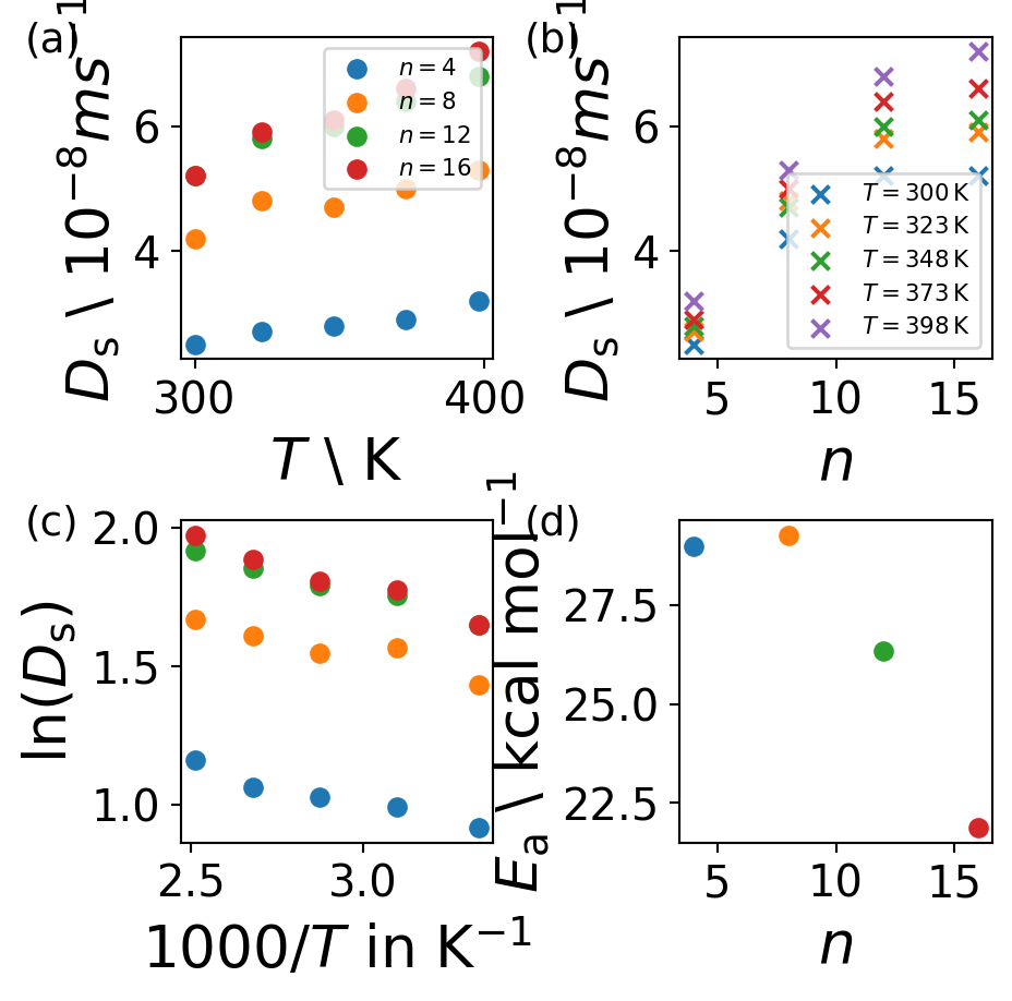
Activation Energy
The diffusion coefficient is directly depending on the activation energy \(E_{\mathrm{a}}\) by an exponential decay \[
D_{\mathrm{s}}=D_0 e^{-\frac{E_{\mathrm{a}}}{RT}}
\] where \(D_0\) is factor of the exponential function, \(R=8.3145\,\mathrm{JK^{-1}mol^{-1}}\) is the ideal gas constant and \(T\) is the temperature.
With this formalism we can apply an Arrhenius equation to fit a linear function to get the activation energy \(E_{\mathrm{a}}\). \[
\ln (D_{\mathrm{s}}) = -\frac{E_{\mathrm{a}}}{RT} + \ln{D_0}
\]
Kubo, R. Statistical-Mechanical Theory of Irreversible Processes. I. General Theory and Simple Applications to Magnetic and Conduction Problems. Journal of the Physical Society of Japan1957, 12 [6], 570–586. https://doi.org/10.1143/jpsj.12.570.